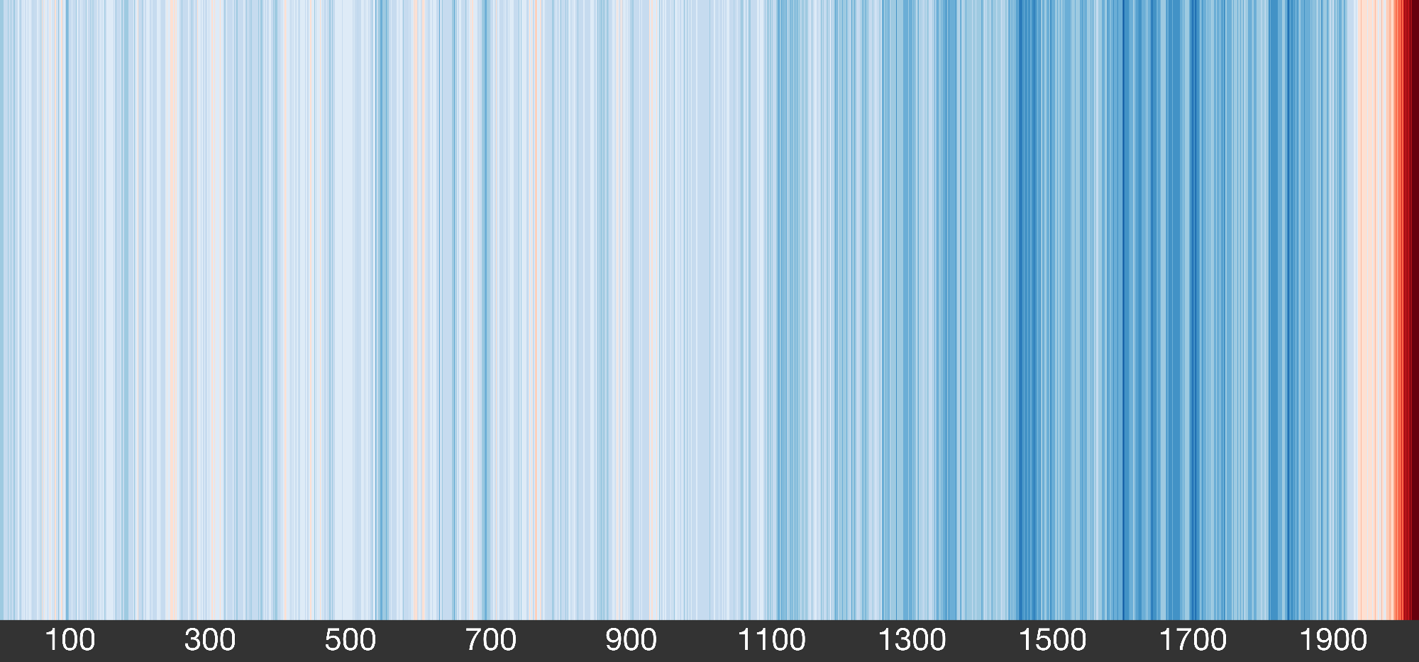
title background: 2022 years of climate stripes relative to the 20th century average, by Ed Hawkins
Now is the summer of our discontent…
(with apologies to Shakespeare’s Richard III)
A Wild Summer
Back in May we noted a “hot start” to 2023, said good-bye to three years of La Niña and speculated that we just might see an El Niño develop later in the year. By mid-June that hot start hit the afterburners, with record high daily average temperatures boosting searing heatwaves and massive wildfire outbreaks. El Niño graduated to a sure thing for 2024. In July we were looking at “global climate chaos“—unprecedented heat worldwide with temperature records on land and in the oceans falling like dominoes, with no end in sight.
Well, here we are in August and the hits just keep on coming. July was crowned the hottest month in recorded history. Sea surface temperatures near the Florida Keys reached an unprecedented 101.19F (38.43C) amid widespread coral bleaching. Florida itself has spent much of the summer under Excessive Heat warnings, as has most of the Southern US. Since March, record-setting wildfires in the hot, dry forests of Northern Canada burned 13.4 million hectares (over 51,737 square miles)—so far. As I write, Canada is fighting 1,135 active fires, with 745 out of control. At the same time, record flooding is happening around the world, from Nova Scotia, to Slovenia, to China.
The Big Picture
With so much going on, it’s easy to get distracted by the parade of meteorological events. Let’s step back and put this summer in context.
Climate scientist Ed Hawkins (University of Reading) used his trademark “climate stripes” to combine the global temperature measurement record (1850 through 2022) with tree ring studies and other paleoclimate data spanning 2022 years. In the resulting chart shown below, the horizontal reference line is the 1900-2000 average temperature. Red stripes are warmer years than the average, blue stripes are cooler. (These stripes are also shown in the title panel of this post.)
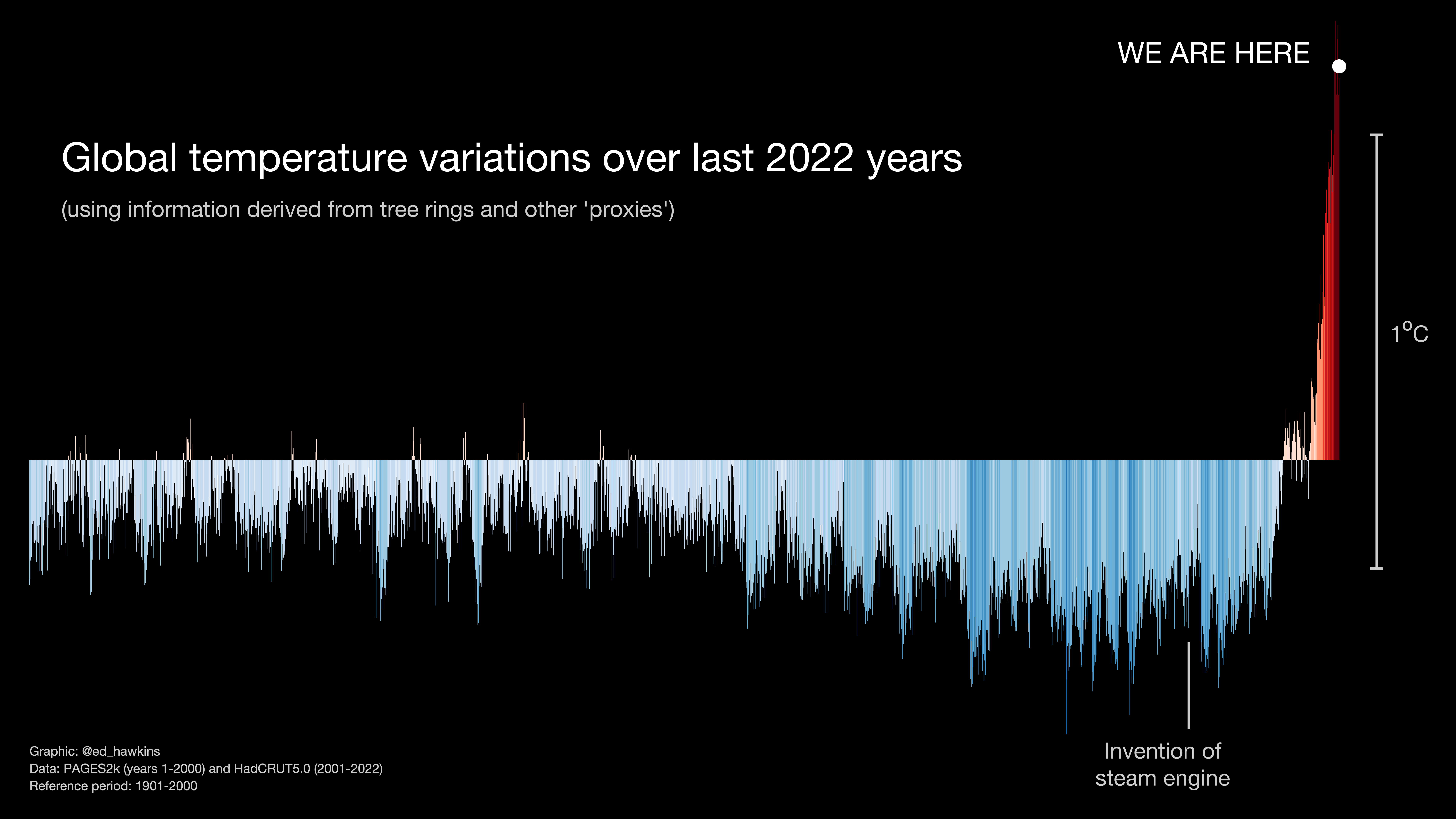
2022 years of climate stripes, referenced to the 20th century average temperature. Credit: Ed Hawkins, University of Reading
The dramatic temperature spike shown to the right of this chart actually puts us outside the temperature envelope in which humanity’s agriculturally based society originated. You need to go back roughly 125,000 years to find temperatures hotter than the chart’s “we are here.”
Let’s zoom in on the recent years and see exactly where we stand after 2023’s record-setting July.
The graph below shows that July was dramatically hotter than in prior years. In fact, July 2023 averaged about 1.5ºC above preindustrial temperatures, giving us our first taste of life at the target goal of the Paris Agreement. Of course, this is a single month—the Paris Agreement target is a sustained global annual average temperature of 1.5ºC above preindustrial levels. Unfortunately, researchers now estimate that there is a 66% chance we will breach the 1.5ºC threshold for an entire year between now and 2027.
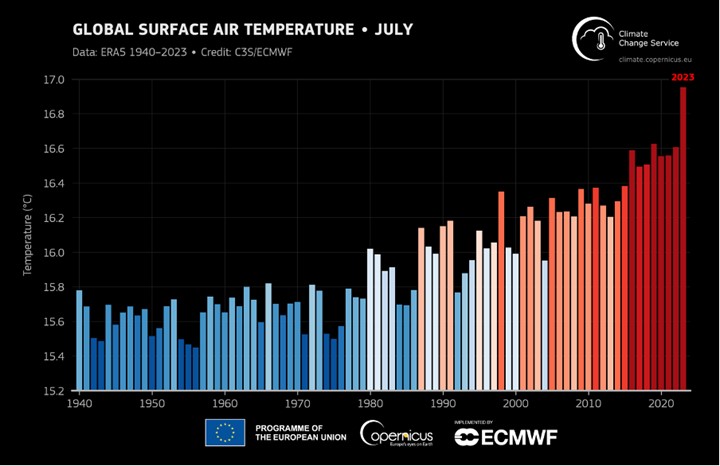
Credit: Copernicus Climate Change Service
The following graph shows just how close we are. Record-breaking temperatures in June and July, and a rapidly developing El Niño led Zeke Hausfather (@hausfath/twitter) and other scientists at Carbon Brief to suggest that 2023 may be the hottest year on record, at an estimated 1.41ºC above the preindustrial level.
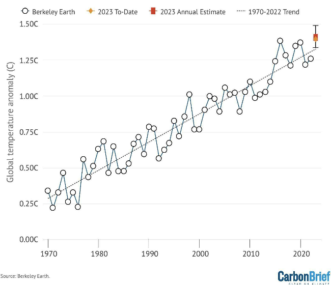
Unfortunately, we are going to blow through the Paris Agreement’s 1.5ºC limit. In fact, without rapid and extensive reduction in greenhouse gas emissions, by 2100 the global average temperature will be roughly 3ºC above preindustrial levels—temperatures last seen millions of years ago.
These climate trends are worrisome enough, but in the meantime rising temperatures are leading to a disproportionate increase in extreme weather events.
How Are Climate Trends Affecting Extreme Weather?
It’s all too tempting to shrug off climate warming predictions like “1.5ºC (2.7ºF) above preindustrial levels.” After all, we see bigger changes than that from one day to the next. Of course, these figures typically refer to global average temperatures over a number of years. Even projected changes in regional or seasonal averages can look deceptively benign. But small changes in an average can lead to disproportionate changes at the margins—in how often we experience extreme weather and in the severity of extreme events.
Temperature is a key indicator of how the climate is changing and how that change may manifest in extreme weather events. Over the past 30 years, atmospheric physicist James Hansen and colleagues have developed and tested a simple and elegant method to show how small changes in global average temperature can greatly affect temperature extremes.
A former director of NASA’s Goddard Institute for Space Studies, Hansen famously introduced the idea of “loaded climate dice” in the late 1980’s to illustrate the increased likelihood of experiencing extreme temperatures in a warming climate. He and his colleagues showed that relatively small increases in the average temperature “load the dice”—changing the odds to favor more frequent and larger temperature extremes. The idea was to show that climate warming, rather than just unusual weather patterns, is the principal cause of increasingly common extreme events.
A thorough discussion of the climate dice investigation and its results can be found here. The following is just a brief summary.
Hansen’s team used actual surface temperature records on a 250km grid, rather than climate model simulations. They chose the thirty-year period from 1951 through 1980 as the basis for their comparisons—a period when the “dice” were not loaded. Global temperatures were relatively stable in that time frame, with rapid warming occurring in subsequent decades. Although some anthropogenic warming had occurred by then, the climate was still within the range to which nature and civilization were adapted. In effect, the 1951-1980 period represented the “climate.”
(This is going to sound like a statistics lecture for a few paragraphs – my apologies!)
Here’s how it works. The following figure shows Northern Hemisphere land summer temperature data for the 1951-1980 reference period and two later decades. Consider the 1951-1980 reference period first – the green curve. This is a typical symmetrical “bell curve.” The peak of the curve is at the mean (average) value for the reference period temperature data. Roughly a third (33%) of the temperature data falls within the white area beneath the curve, and the width of the white area defines “1 standard deviation” or “1 sigma.” (On the x-axis “anomaly” or sigma scale the white zone is between +0.5 and -0.5) As we move to temperatures left or right (cooler or warmer) of the central white area, we find progressively fewer and fewer data points, and the curve tapers off with a small number of the coldest and the warmest observations.
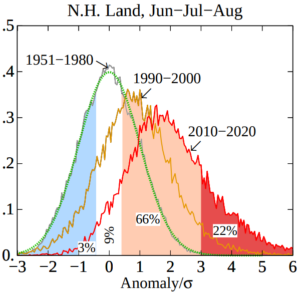
The effect of warming climate on extreme heat events. Source: James Hansen
Remember the standard deviation? Well, it turns out that statistics says 99.7% of the temperature data fall within three standard deviations of the mean (between -3 and +3 on the graph.) Not only that – it also means that 0.15% of the data is colder than the -3 sigma value. Similarly, 0.15% is hotter than +3 sigma. Since our curve is symmetrical, roughly 33% of the data falls within each of the blue (cooler than average temperatures) and the pink (warmer than average) regions under the green curve. The standard deviations, -1 to -3 to the left of the mean and 1 to 6 to the right, define negative (cooler) or positive (warmer) anomalies. Note that all anomalies are relative to the 1951-1980 reference period (the green curve).
Now we get to the good stuff. The yellow curve represents the 1990-2000 temperature data, while the red curve represents 2010-2020. Both curves appear less smooth than the green curve because there are only 10 years worth of data in each, vs. 30 years for the reference period. The curves are “normalized” so the single decade data can be compared with the three decade base data.
Let’s compare! The first thing we see is that the yellow curve is lower than the green curve of our climate baseline, and the red curve is lower still. This is because the yellow and red curves are wider than the green curve—our new climates are more variable than the baseline. The next thing we notice is that the mean temperatures are warmer (the peak of the curve has moved to the right). Climate warming is starting to load the dice.
If we look at the red curve, we see that 66% of the data fall in the pink zone, within +3 sigma of the 1951-1980 “climate” mean. If you grew up between 1951 and 1980, you were unlikely to see a day with temperatures higher than the pink zone, and even they only happened 33% of the time. Now, in 2010-2020 they happen 66% of the time—the number of what you thought of as hot days has doubled. The cool summer days (blue zone) in 1951-1980 happened 33% of the time, but now only 3% of the time. The goldilocks days in the white zone? Only 9% of the time in 2010-2020.
So, that’s what we would expect with climate warming, right? Yes, but… we also get extreme weather, in the form of unprecedented heat.
That dark red area beyond the 3 sigma anomaly constitutes 22% of the 2010-2020 data, likely representing weather hotter than you ever experienced between 1951 and 1980. To be accurate, greater than 3 sigma events were possible back then, but very unlikely. Now, 22% of the data represents heat that was virtually impossible before 2010-2020. The dramatic increase in these extreme anomalies suggests that extreme events like 2023’s heatwaves in Europe and the southern US are clearly a consequence of climate warming. Some meteorologists or climate warming skeptics may reject global warming as the cause of such events (“We’ve had heat waves before. It’s just another high pressure ridge” or “It’s El Niño”.) Hansen points out that these weather patterns have always been common, but the large areas of extreme heat we are experiencing have only come into existence with global climate warming.
Attribution Science and Extreme Weather
Further bolstering climate warming as the proximate cause of extreme weather events is the evolving discipline of attribution science. Hansen’s data driven approach is best suited to retrospective analysis of large areas for past events and long term trends. Attribution science is more dynamic.
The World Weather Attribution organization (WWA) is a network of scientists using weather data and climate models to understand how climate warming influences the intensity and likelihood of extreme weather events. Their objective is to perform these analyses rapidly – even while the event is ongoing.
With heatwaves plaguing many countries early this summer, WWA launched a study to determine the possible role of climate change in heatwaves early in July 2023:
- western US, Texas and northern Mexico (July 1-18)
- southern Europe (July 12-18)
- the lowlands of China (July 5-18)
These extreme weather events continued beyond the study period. Nonetheless, WWA was able to determine the degree of connection between climate change and each of the events. The key results:
- The 2023 heat waves are not rare in today’s climate. On average, we can expect the US/Mexico heatwave to be a 1 in 15 year event, the Southern Europe event 1 in 10 years, and the lowland China heatwave 1 in 5 years.
- In the absence of climate change these events would be “extremely rare” – a 1 in 250 year event in China. The US/Mexico and Southern Europe events would have been “virtually impossible” without climate change.
- Climate change also made the heatwaves hotter: 2.5ºC warmer in Southern Europe, 2ºC warmer in the US/Mexico region, and about 1ºC in China
- These results reflect the current level of climate warming, roughly 1.2ºC above preindustrial temperatures. At higher levels of warming WWA projects that these heat events will be more frequent, hotter, and longer lasting. Heatwaves like these would occur every 2-5 years with temperatures 2ºC above preindustrial levels.
Some of these events were still ongoing when the attribution study began. It’s not clear at this writing if the final scale of the events will affect the results, but the telltale fingerprint of climate change will remain regardless.
Future Trends in Extreme Weather
Hansen et al suggest that the recent deviation of the global warming curve from the 0.18ºC/decade line shown in the figure below is at least partly attributable to the reduction in aerosols, and that we are entering a period of accelerated warming, somewhere between 0.27ºC/decade and 0.36ºC/decade (respectively the lower and upper boundaries of the yellow area in the graph.)
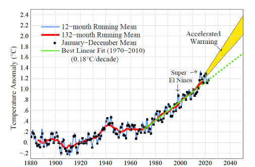
Projected rates of warming with reduced aerosols
If this hypothesis holds true, without major reductions in greenhouse gas emissions we will pass the 1.5ºC target in the late 2020’s and 2ºC in the early 2040’s.
It looks like we may have less time than we thought to get climate warming under control. We’ll keep you posted as this concept gets tested. Stay tuned!